Theoretical Background
Numerical method framework
Governing equations
The governing equations are the forced incompressible Navier-Stokes equations:
where \(\mathbf{u}\) is the velocity field, \(p\) is the pressure field, \(\nu\) is the kinematic viscosity, and \(\mathbf{f}\) is the external force field. Eq. (1) is the momentum equation and Eq. (2) is the incompressibility constraint. Further details on the numerical methods can be found in [1, 2, 3].
Time advancement
The time advancement of Eq. (1) can be expressed as:
with
and
for a Runge-Kutta scheme with coefficients \(a_k\), \(b_k\), and \(c_k=a_k+b_k\) and \(n_k\) sub-time steps \(k=1,\dots{n_k}\) with \(t_1=t_n\) and \(t_{n_k} = t_{n+1}\). Pressure and forcing terms are expressed through their time-averaged values on a given sub-step \(c_k\Delta{t}\), indicated by the tilde in \(\tilde{p}^{k+1}\) and \(\tilde{\mathbf{f}}^{k+1}\).
Boundary conditions
The governing equations Eq. (1) and (2) are solved in a computational domain \(L_x \times L_y \times L_z\) discretised on a Cartesian mesh of \(n_x \times n_y \times n_z\) nodes.
At the boundaries of the time periodic, free-slip, no-slip, or open conditions can be applied depending on the flow configuration considered. Period and free-slip boundary conditions can be imposed directly via the spatial discretisation without specific care in time advancements.
However, the use of Dirichlet conditions on the velocity (for no-slip or open conditions) needs to be defined according to time advancement procedure. Conventional homogeneous Neumann conditions are used to solve the pressure.
Role of intermediate velocities
In this approach, we introduce two intermediate velocities \(\mathbf{u}^*\) and \(\mathbf{u}^{**}\). The motivation for using these intermediate steps is to enforce the divergence-free condition at the walls while also satisfying Dirichlet boundary conditions.
First, we compute a velocity field \(\mathbf{u}^*\) that satisfies the momentum equation without yet enforcing incompressibility. This provides a preliminary estimate of the velocity. Next, we modify \(\mathbf{u}^*\) by incorporating the pressure gradient from the previous time step \(\nabla{p}^k\) to obtain \(\mathbf{u}^{**}\).
To ensure \(\nabla\cdot\mathbf{u}^{k+1}=0\) we use the pressure gradient \(\nabla{p}^{k+1}\) from the current time-step:
At the walls, \(\mathbf{u}^*\big|_w=0\) (no-slip condition for the first intermediate velocity) which when substituted into Eq. (6) gives:
Therefore, the velocity at the wall in the current time-step is:
Since for small time steps \(\nabla{p}^{k+1}\approx\nabla{p}^{k}\) this results in:
which ensures that the no-slip boundary condition is satisfied.
Pressure treatment
The incompressibility condition (2) can be verified at the end of each sub-time step \(\nabla\mathbf{u}\cdot\mathbf{u}^{k+1} =0\) through the solving of a Poisson equation:
that provides the estimation of \(\tilde{p}^{k+1}\) required to perform the pressure correction.
Spatial discretisation
Convective and viscous terms
Assuming that we have a uniform distribution of \(n_x\) nodes \(x_i\) on the domain \([0, L_x]\) with \(x_i=(i-1)\Delta{x}\) for \(1\le{i}\le{n_x}\), the first derivative \(f'(x)\) of the function \(f(x)\) can be approximated by a finite difference scheme of the form:
By choosing \(\alpha=1/3\), \(a=14/9\), \(b=1/9\) this approximation is sixth-order accurate while having a so-called “quasi-spectral behaviour” due to its capabilities to represent accurately a wide range of scales. The compromise of the sixth-order accuracy has been chosen to maintain a compact formulation via the use of a Hermitian structure of the scheme with \(\alpha\ne{0}\). Even though this scheme is twice as expensive as a second-order scheme, in order to get the same solution with second-order scheme will require four to five times more mesh nodes.
Pressure
Convective and diffusive terms are discretised using scheme (12) on a collocated mesh whereas a partially staggered mesh is used for the pressure treatment. To evaluate \(f'_{i+1/2}\) of the first derivative at the staggered nodes by a half-mesh \(\Delta{x}/2\), the sixth-order finite-difference scheme can be expressed as:
with \(\alpha=9/62\), \(a=63/62\) and \(b=17/62\). The spectral behaviour of this scheme is better than its collocated counterpart (12).
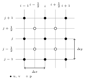
Arrangement of variables in 2D for a partially staggered grid.
Assuming that \(f\) is periodic over the domain \([0,L_x]\), the discrete Fourier transform of the function \(f\) can be expressed as:
where \(l=\sqrt{-1}\) and \(k_x=2\pi{l}/L_x\) is the wave number. The inverse discrete Fourier transform is given by:
It can be shown that the Fourier coefficients \(\hat{f}'_l\) associated with the approximation (12) are linked to the Fourier coefficients \(\hat{f}_l\) given by (14) by the simple spectral relation:
where \(k'_x\) is the modified wave number related to the actual wave number \(k_x\) by
The concept of the modified wave number still holds in the staggered formulation, and the expression of \(k'_x\) associated with the scheme (13) is given by:
The well known principle of equivalence between multiplication in Fourier space and derivation/interpolation in the physical space is recalled here. This equivalence is exact, hence, the computation of a derivative in physical space using (13) with relevant boundary conditions must lead to the same result obtained with the use of (18) in spectral space.
Solving the Poisson equation
There are several numerical algorithms for solving Poisson’s equations, which can be broadly classified into two categories: iterative solvers and direct solvers. x3d2 currently uses direct methods with iterative solvers planned in future versions. Among the direct methods, Fast Fourier Transform (FFT) based solvers are the most efficient.
For simplicity, a generic 3D Fourier transform can be defined as:
with its inverse expression
where the sums, the base functions \((W_x, W_y, W_z)\) and the wave numbers \((k_x, k_y, k_z)\) can correspond to standard FFT (for periodic boundary conditions) or cosine FFT (for free-slip or \(\mathbf{u}\)-Dirichlet/\(p\)-Neumann boundary conditions) in their collocated or staggered versions. 3D direct (19) and inverse (20) can be performed with any efficient FFT routines available in scientific Fortran or C libraries. The first stage in solving the Poisson equation (11) consists in the computation of its right-hand side. After performing the relevant Fourier transform (19) to \(D=\nabla\cdot\mathbf{u}^{**}\), the solving of the Poisson equation consists in a single division of each Fourier mode \(\hat{D}_{lmn}\) by a factor \(F_{lmn}\) with
where the expression of this factor depends on the mesh configuration. For instance, in the case of a partially staggered approach, the factor \(F_{lmn}\) must take the mid-point interpolation into account through the use of a transfer function with the following form:
where \(T_x(k_x\Delta{x})\) is the transfer function related to the wave number \(k_x\) by
Stretched mesh in one direction
The pressure discretisation described so far is only valid for a regular mesh in three spatial directions. To overcome this difficulty a modification of the Poisson solver is proposed which is based on a specific function mapping and expressed using only few Fourier modes. This approach preserves the spectral and non-iterative nature of the pressure treatment without significant loss of accuracy.
For simplicity consider a one-dimensional problem where \(y\) is the physical coordinate and \(s\) is the computational coordinate:
where \(h(s)\) is the mapping from equally spaced coordinate \(s\) to the stretched physical coordinate \(y\). The derivatives with respect to \(y\) can be estimated using the chain rule, where the first derivative is given by:
and the second derivative is given by:
Expressed in physical space, these rules can be used to implement schemes like (12) and (13) where the finite differences are performed on the regular coordinate \(s\) (instead of \(x\)).
The main difficulty is in the treatment of the Poisson equation that requires similar operations in the spectral space. Here the metric \(1/h'\) is expressed with only three Fourier modes in spectral space:
so that the mapping (24) can be written as:
where \(H\) is the Heaviside step function. This mapping preserves the accuracy while avoiding expensive computation of a full convolution and ensuring the strict physical/spectral equivalence.
\(\alpha=0\), \(\gamma=1\) and \(\delta=0\) the mapping leads to refinement in the centre of an infinite domain
\(\alpha\ne{0}\), \(\gamma=1\) and \(\delta=0\) leads to refinement in the centre of a finite domain
\(\gamma=1\) and \(\delta=1/2\) leads to refinement near the boundaries for a finite domain (not compatible with periodic boundary conditions) because \(1/h'\) is not periodic over \(L_y\)
\(\gamma=1/2\) and \(\delta=1/2\) leads to refinement near the bottom boundary only for a finite domain
It can be deduced that the three coefficients of the metric (28) are non-zero with
for \(\gamma=1\) and \(\delta=0\) or \(1/2\). The main advantage of this compact expression in spectral space is that the convolution of the metric by the first derivation with respect to the regular coordinate \(s\) requires only \(3n_y\) multiplications.
To solve the Poisson equation (11) (using 3D Fourier transforms (19) and (20) where \(y\) needs to be substituted by \(s\) for the \(y\)-stretched approach) the counterpart of the integration scheme (21) becomes
where \(\hat{\tilde{\mathbf{p}}}_{ln}^{k+1}\) and \(\widehat{\mathbf{D}}_{ln}\) are \(n_y\) vectors of components of \(\hat{\tilde{p}}_{ln}^{k+1}\) and \(\widehat{D}_{ln}\) and \(\mathbf{B}\) is a \(n_y \times n_y\) pentadiagonal matrix of components. For the partially staggered case these components are:
where the \(k'_m\) are the modified wave numbers from relation like (17) or (18) based on the computational coordinate \(s\) instead of \(x\).
The above matrix is diagonal for a regular \(y\)-coordinate (with \(a_1=a_{-1}=0\)) so that the simplified expression (23) can be recovered. In the other cases, the computation of pressure nodes \(\hat{\tilde{\mathbf{p}}}_{ln}^{k+1}\) requires inverting \(n_x \times n_y\) linear systems based on \(n_y\times{n_y}\) pentadiagonal matrices. The corresponding computational cost is proportional to \(n_x\times{n_y}\times{n_z}\) so that the solver Poisson can be direct without any iterative process.
In terms of computational cost, solving the Poisson equation directly requires both a forward and an inverse 3D FFT. For a completely regular mesh in three spatial dimensions, these two FFT operations constitute the majority of the computational expense for the Poisson stage, accounting for about 10% of the total computational effort required to solve the Navier-Stokes equations. When dealing with meshes that have one stretched direction, the cost of ensuring incompressibility increases but still represents about 15% of the overall computational cost for a given simulation.
Although using Fourier transforms for pressure is highly suitable for periodic or free-slip boundary conditions, it is less ideal for no-slip or open boundary conditions. In these cases the pressure must be expressed using cosine Fourier transforms, assuming that homogeneous Neumann conditions are met. This assumption introduces an error that is only second-order accurate in space.
Tridiagonal systems
A tridiagonal system is a linear system of equations where the non-zero coefficients are concentrated along the main diagonal, the subdiagonal, and the superdiagonal. These systems frequently occur in high-order compact finite difference schemes and take the form \(Ax=d\):
where \(a_0=c_{N-1}=0\).
Tridiagonal systems solver algorithms
The Thomas algorithm is a well-known method for solving tridiagonal systems of equations. It is a specialised form of Gaussian elimination that involves a forward pass to eliminate the lower diagonal elements \(a_i\) of the tridiagonal matrix by adding a multiple of the row above, followed by a backward substitution pass using the modified upper diagonal coefficients \(c_i\). Even though the Thomas algorithm is inherently serial, when solving a batch of tridiagonal systems it is possible to parallelise the overall operation by assigning many tridiagonal systems per MPI rank.
However, the Thomas algorithm requires the entire length of a tridiagonal system to be contained within a single rank. Consequently, this strategy necessitates MPI all-to-all communication to rearrange the domain decomposition, ensuring that batches of tridiagonal systems are oriented in the \(x-\), \(y-\), and \(z-\) directions. This ensures that the entire length of each tridiagonal system is always within a single rank, while individual systems are distributed across all available ranks. As a result, the derivations and interpolations can be performed in each direction using the Thomas algorithm.
The fundamental difference between a serial algorithms like Thomas algorithm and distributed-memory algorithms is that the distributed algorithms divide the individual systems into multiple subdomains. This enables localised communication (e.g. neighbour-to-neighbour exchanges) instead of global dependencies. For example, a 3D decomposition strategy can distribute subdomains across ranks while maintaining static decomposition states, avoiding frequent reconfiguration. Crucially, these approaches eliminate the need for MPI all-to-all communications across the entire domain.
Many tridiagonal algorithms face performance challenges, particularly along the \(x\) direction, due to inefficient memory access patterns in Cartesian data structures. There are two main characteristics in tridiagonal matrix algorithms that are crucial for computational performance:
The algorithms are heavily bandwidth-bound because the FLOP requirements of these algorithms are very low compared to the data movement requirements.
The backward and forward passes of the algorithm require accessing the same data twice in a short time interval. This can be optimised by using CPU cache or GPU shared memory to store intermediate states between the forward and backward passes.
x3d2’s solution: DistD2-TDS
To address the challenges of solving tridiagonal systems efficiently in distributed-memory environments on both CPUs and GPUs, x3d2 uses a novel algorithm called DistD2-TDS (see [4] for more details). This algorithm is based on a specialised data structure that:
Improves data locality and minimises data movements via cache blocking and kernel fusion strategies.
Enables a contiguous data access pattern, resulting in efficient utilisation of the available memory bandwidth.
Supports vectorisation on CPUs and thread-level parallelisation on GPUs for improved performance.
Modern CPUs have large enough caches to store the entire tridiagonal matrix, which can be accessed quickly. However, GPU caches are not large enough, and kernel fusion is the only option to reduce data movement on GPUs. To enable a linear and predictive memory access pattern regardless of the spatial direction of the tridiagonal systems, DistD2-TDS data structure subdivides the computational domain into groups of individual tridiagonal systems. These groups are tightly packed in memory to ensure data continuity. This arrangement enables vectorisation on CPUs and thread-level parallelism on GPUs, as the \(n^{th}\) entries of all tridiagonal systems within a group are stored next to each other in memory. Therefore, the sequential operations in the algorithms, as we apply the forward and backward passes, can be concurrently executed for \(SZ\) systems at once per core on a CPU or per SM on a GPU.
Example: In a domain of size \(32 \times 8 \times 4\) shown below; a single group consist of 4 individual tridiagonal systems, resulting in 8 groups in total. For a Cartesian mesh with \(n_x\), \(n_y\), and \(n_z\) the data is arranged as \(SZ, n_x, n_y \cdot n_z / SZ\) for an \(x\)-directional layout where \(SZ\) is the number of tridiagonal systems in a group.
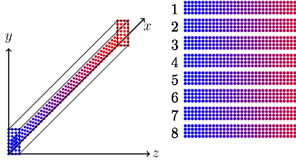
x3d2 data structure for an \(x\)-directional tridiagonal system. Data continuity in memory is in column-major order.
Typically, for a double-precision simulation on CPUs, \(SZ=8\) as vector registers (512 bits) handle 8 double-precision FLOPs per cycle. For GPUs, \(SZ=32\) as a single streaming multiprocessor (SM) typically has 32 double-precision cores in total, where each core is effectively assigned an individual tridiagonal system.
Tridiagonal systems resulting from high-order compact finite-difference schemes are always diagonally dominant, and the algorithm used in x3d2 takes advantage of this characteristic to minimise communication requirements between ranks. This involves dividing a batch of tridiagonal systems into multiple domains, where the subdomains are located across multiple ranks in a distributed memory environment.
Apart from the specialised data structure in DistD2, another novel aspect of this algorithm is that it fuses the RHS construction based on discretised equations such as Eq. (12) with the forward pass in the decoupling phase of the algorithm – this minimises data movement requirements.
After the decoupling phase of the algorithm, the next step is to solve the reduced system. By exploiting diagonal dominance, certain entries in the reduced system can be eliminated without any loss in numerical accuracy, leading to independent \(2 \times 2\) systems that are coupled across MPI boundaries. This step is the main deviation from other tridiagonal solvers that use a PCR-type strategy to obtain the solution of the reduced system on a single rank. In the DistD2 algorithm, the reduced systems are not coupled across the entire domain, but only across 2 individual ranks across an MPI boundary. These smaller systems are then solved efficiently using local communication between neighbouring ranks. This single-step MPI communication involving two neighbouring ranks is a significant advantage of the DistD2 algorithm over existing strategies. Finally, the substitution phase of the algorithm requires a simple algebraic substitution and does not require any further MPI communications.
2D Domain Decomposition for FFT
The current implementation of x3d2 uses a direct approach, namely Fast Fourier Transform (FFT), to solve the Poisson equation. Spectral codes often involve performing FFTs along global mesh lines. There are two approaches to performing such computations on distributed-memory systems:
Develop distributed algorithms (such as a parallel tridiagonal solver or parallel FFT working on distributed data).
Dynamically redistribute (transpose) data among processors to apply serial algorithms in local memory.
The second approach is often preferred due to its simplicity. Many applications have implemented this idea using 1D domain decomposition. However, 1D decomposition has some limitations. For example, for a cubic mesh size of \(N^3\), the maximum number of processors \(N_{\mathrm{proc}}\) that can be used in a 1D decomposition is \(N\), as each slab must contain at least one plane. For a cubic mesh of 1 billion points, this constraint is \(N_{\mathrm{proc}} \lt 10^4\). This limitation can be overcome by using 2D domain decomposition. While a 1D decomposition algorithm swaps between two states, a 2D decomposition requires traversing three different states using four global transpositions to complete a cycle. The swapping between states can be achieved using the MPI_ALLTOALL(V) library.

1D domain decomposition (left), 2D domain decomposition (middle), 3D domain decomposition (right).
2D domain decomposition is widely used for spectral codes, particularly those compatible with implicit schemes in space. This method allows for efficient parallelization by dividing the computational domain into smaller subdomains, each handled by a separate processor. For a simulation with a cubic mesh of size \(N^3\), up to \(N^2\) processors can be used, significantly increasing scalability compared to 1D decomposition.
x3d2 uses the 2DECOMP&FFT library for 2D decomposition and FFT (see [5] for more details) when using OpenMP as a backend (for NVIDIA GPUs it uses cuFFT). One of the key advantages of using the 2DECOMP&FFT library is that it does not require modifications to the existing derivative and interpolation subroutines, making it easier to implement. Additionally, this approach utilises customised global MPI_ALLTOALL(V) transpositions to redistribute data among processors. Although communication overhead can range from 30% to 80% of the total computational time, with up to 70 transpositions per time step, the overall efficiency and scalability of the simulations are greatly enhanced.
References
P. Bartholomew, G. Deskos, R. A. S. Frantz, F. N. Schuch, E. Lamballais, and S. Laizet. Xcompact3D: An open-source framework for solving turbulence problems on a Cartesian mesh. SoftwareX, 12:100550, 2020. doi:10.1016/j.softx.2020.100550.
S. Laizet and E. Lamballais. High-order compact schemes for incompressible flows: A simple and efficient method with quasi-spectral accuracy. Journal of Computational Physics, 228(16):5989–6015, 2009. doi:10.1016/j.jcp.2009.05.010.
E. Lamballais, V. Fortuné, and S. Laizet. Straightforward high-order numerical dissipation via the viscous term for direct and large eddy simulation. Journal of Computational Physics, 230(9):3270–3275, 2011. doi:10.1016/j.jcp.2011.01.040.
S. Akkurt, S. Lemaire, P. Bartholomew, and S. Laizet. A Distributed-memory Tridiagonal Solver Based on a Specialised Data Structure Optimised for CPU and GPU Architectures. (preprint), 2024. doi:10.48550/arXiv.2411.13532.
N. Li and S. Laizet. 2DECOMP & FFT-a highly scalable 2d decomposition library and FFT interface. In Cray User Group Proceedings, 1–13. 2010.